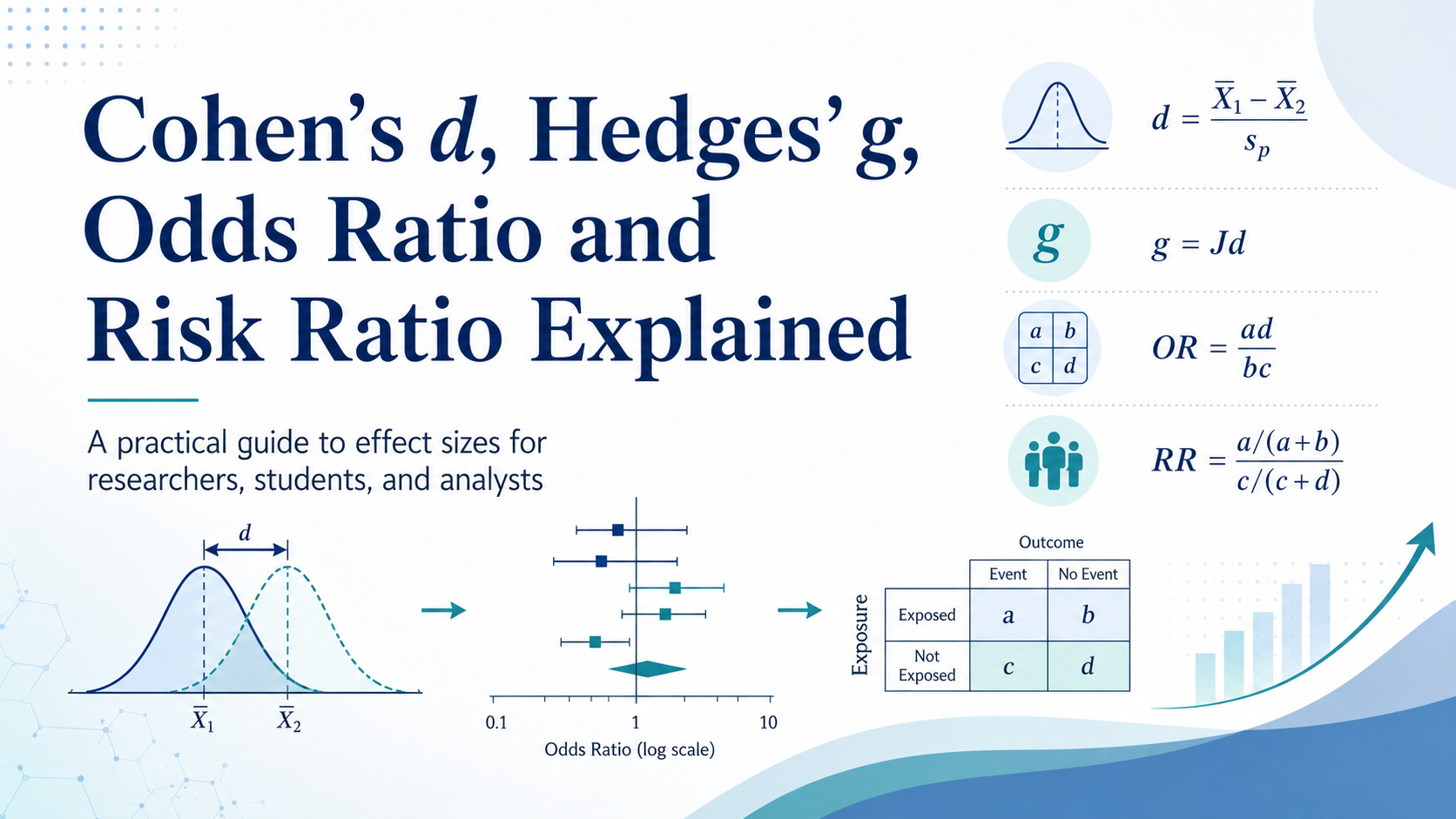
Cohen’s d, Hedges’ g, odds ratio, and risk ratio are four commonly used effect-size measures. Cohen’s d and Hedges’ g quantify differences between group means for continuous outcomes, while the odds ratio and risk ratio compare binary outcomes such as success versus failure, recovery versus no recovery, or disease versus no disease.
Choosing the correct effect-size measure is essential because statistical significance alone does not tell you how large or practically important an effect is. A very small difference can become statistically significant in a large sample, while a meaningful effect may fail to reach significance in a small study.
This guide explains:
- What Cohen’s d, Hedges’ g, odds ratio, and risk ratio mean
- How each measure is calculated
- How to interpret their values
- When to use each effect size
- Why odds ratios and risk ratios are not interchangeable
- Which measures are commonly used in meta-analysis
- Common mistakes researchers should avoid
Quick Comparison: Cohen’s d vs Hedges’ g vs Odds Ratio vs Risk Ratio
| Effect-size measure | Outcome type | What it compares | Null value | Common use |
|---|---|---|---|---|
| Cohen’s d | Continuous | Difference between two means in standard-deviation units | 0 | Experiments, psychology, education, behavioral science |
| Hedges’ g | Continuous | Bias-corrected standardized difference between two means | 0 | Meta-analysis and studies with small samples |
| Odds ratio | Binary | Odds of an event in one group relative to another | 1 | Logistic regression, case-control studies, meta-analysis |
| Risk ratio | Binary | Probability of an event in one group relative to another | 1 | Randomized trials, cohort studies, clinical research |
The most important distinction is the type of outcome:
- Use Cohen’s d or Hedges’ g when the outcome is continuous, such as blood pressure, test scores, pain ratings, or income.
- Use an odds ratio or risk ratio when the outcome is binary, such as whether an event occurred.
The Cochrane Handbook classifies standardized mean differences as measures for continuous outcomes and risk ratios and odds ratios as relative measures for dichotomous outcomes.
What Is an Effect Size?
An effect size is a numerical measure of the magnitude and direction of a difference, relationship, or treatment effect.
A p-value addresses a question such as:
If there were no real effect, how compatible would the observed data be with that assumption?
An effect size addresses a different question:
How large is the observed difference or association?
For example, suppose an intervention produces a statistically significant improvement in examination scores. The p-value indicates the strength of evidence against the null hypothesis, but it does not tell you whether the improvement was 0.5 points, 5 points, or 20 points.
An effect size provides that missing information.
Effect estimates should normally be reported with a measure of uncertainty, particularly a confidence interval. A confidence interval helps readers evaluate both the estimated magnitude of the effect and the precision of that estimate.
Cohen’s d Explained
What Is Cohen’s d?
Cohen’s d is a standardized mean difference that expresses the difference between two group means in standard-deviation units.
For two independent groups, Cohen’s d is commonly calculated as:
$$
d =
\frac{\bar{X}_1-\bar{X}_2}{s_p}
$$
where:
- $\bar{X}_1$ is the mean of Group 1
- $\bar{X}_2$ is the mean of Group 2
- $s_p$ is the pooled standard deviation
The pooled standard deviation is:
$$
s_p =
\sqrt{
\frac{
(n_1-1)s_1^2+(n_2-1)s_2^2
}{
n_1+n_2-2
}
}
$$
where:
- $n_1$ and $n_2$ are the group sample sizes
- $s_1$ and $s_2$ are the group standard deviations
Because Cohen’s d is standardized, it has no original measurement unit. A Cohen’s d of 0.60 means that the two group means differ by approximately 0.60 pooled standard deviations.
Example of Cohen’s d
Suppose researchers compare examination scores between students using a new learning system and students receiving standard instruction.
| Group | Sample size | Mean score | Standard deviation |
|---|---|---|---|
| New learning system | 40 | 80 | 10 |
| Standard instruction | 35 | 74 | 8 |
First, calculate the pooled standard deviation:
$$
s_p =
\sqrt{
\frac{
(40-1)(10^2)+(35-1)(8^2)
}{
40+35-2
}
}
$$
$$
s_p =
\sqrt{
\frac{
3900+2176
}{
73
}
}
\approx 9.12
$$
Then calculate Cohen’s d:
$$
d =
\frac{80-74}{9.12}
\approx 0.66
$$
The mean score in the intervention group was therefore approximately 0.66 standard deviations higher than the mean score in the comparison group.
How to Interpret Cohen’s d
Frequently cited benchmarks proposed by Cohen are:
| Absolute value of d | Conventional description |
|---|---|
| 0.20 | Small effect |
| 0.50 | Medium effect |
| 0.80 | Large effect |
These values are only general conventions. They are not universal rules.
A Cohen’s d of 0.20 may be important when:
- The outcome is serious
- The intervention is inexpensive
- The treatment can be applied to a large population
- Small individual effects accumulate over time
A Cohen’s d of 0.80 may be less important if the intervention is costly, risky, or difficult to implement.
Interpretation should therefore consider the research field, measurement reliability, baseline variation, costs, benefits, and practical consequences.
What Does the Sign of Cohen’s d Mean?
The sign indicates the direction of the difference.
If Cohen’s d is calculated as:
$$d=\frac{\bar{X}_{\mathrm{treatment}}-\bar{X}_{\mathrm{control}}}{s_p}$$
then:
- A positive value means the treatment group had the higher mean.
- A negative value means the control group had the higher mean.
- A value of zero means the group means were equal.
The sign is only meaningful when the order of subtraction and the direction of the outcome scale are clearly defined.
For example, a negative effect could represent either harm or benefit. A lower depression score may indicate improvement, whereas a lower quality-of-life score may indicate deterioration.
When Should You Use Cohen’s d?
Cohen’s d is generally appropriate when:
- You are comparing two group means
- The outcome is continuous
- The groups are independent
- The standard deviations are reasonably comparable
- The sample is large enough that small-sample bias is not a major concern
Common examples include:
- Treatment versus control
- Online learning versus classroom instruction
- Two teaching methods
- Two user-interface designs
- Exposed versus unexposed groups
- Experimental versus baseline conditions
Limitations of Cohen’s d
Cohen’s d is affected by the standard deviation used in its denominator.
Two studies may report the same raw mean difference but different Cohen’s d values if their participant variability differs. This can make interpretation difficult when study populations are substantially different.
The standardized mean difference also assumes that differences in standard deviations primarily reflect differences in measurement scales rather than meaningful differences in population variability. Cochrane therefore recommends caution when combining studies whose populations have genuinely different levels of variation.
Cohen’s d may also be positively biased in small samples, meaning that its absolute value can slightly overestimate the underlying population effect. Hedges’ g is designed to reduce this bias.
Hedges’ g Explained
What Is Hedges’ g?
Hedges’ g is a standardized mean difference similar to Cohen’s d, but it includes a correction for small-sample bias.
A common calculation begins with Cohen’s d and multiplies it by a correction factor:
$$
g = Jd
$$
An approximate correction factor is:
$$
J =
1-
\frac{3}{4df-1}
$$
where:
$$
df=n_1+n_2-2
$$
Therefore:
$$
g =
\left(
1-
\frac{3}{4(n_1+n_2-2)-1}
\right)d
$$
The exact correction can also be expressed using gamma functions:
$$
J(df)=
\frac{
\Gamma(df/2)
}{
\sqrt{df/2},
\Gamma((df-1)/2)
}
$$
For most practical applications, the approximation is sufficiently accurate.
Example of Hedges’ g
Suppose a study reports:
$$
d=0.70
$$
with:
$$
n_1=20
$$
and:
$$
n_2=20
$$
The degrees of freedom are:
$$
df=20+20-2=38
$$
The correction factor is:
$$
J=
1-
\frac{3}{4(38)-1}
$$
$$
J=
1-
\frac{3}{151}
\approx 0.980
$$
Hedges’ g is:
$$
g=0.980\times0.70\approx0.69
$$
The corrected effect is slightly smaller than Cohen’s d.
As the total sample size increases, the correction factor approaches 1. Consequently, Cohen’s d and Hedges’ g become nearly identical in large samples.
Cohen’s d vs Hedges’ g
| Feature | Cohen’s d | Hedges’ g |
|---|---|---|
| Outcome type | Continuous | Continuous |
| Standardized | Yes | Yes |
| Uses pooled standard deviation | Usually | Usually |
| Corrects small-sample bias | No | Yes |
| Common in individual studies | Yes | Yes |
| Common in meta-analysis | Sometimes | Frequently |
| Null value | 0 | 0 |
When Should You Use Hedges’ g?
Hedges’ g is usually preferred when:
- One or more studies have small sample sizes
- You are conducting a meta-analysis
- Studies use different instruments to measure the same construct
- You want a less biased estimate of the standardized mean difference
For example, a depression meta-analysis may include studies using several different depression scales. The raw mean differences cannot be directly combined because the scales have different units. Hedges’ g places the results on a common standard-deviation scale.
The standardized mean difference used in Cochrane reviews corresponds to Hedges’ adjusted g, using a pooled standard deviation and a small-sample correction.
How to Interpret Hedges’ g
Hedges’ g is interpreted in the same standard-deviation units as Cohen’s d.
For example:
- $g=0$ indicates no standardized mean difference.
- $g=0.30$ indicates a difference of 0.30 standard deviations.
- $g=-0.75$ indicates that the first group’s mean is 0.75 standard deviations below the second group’s mean.
The conventional small, medium, and large benchmarks are sometimes applied to Hedges’ g, but contextual interpretation remains more important than arbitrary thresholds.
Risk Ratio Explained
What Is a Risk Ratio?
The risk ratio compares the probability of an event in one group with the probability of the same event in another group.
It is also called the relative risk.
Consider the following $2\times2$ table:
| Event | No event | Total | |
|---|---|---|---|
| Treatment or exposed group | $a$ | $b$ | $a+b$ |
| Control or unexposed group | $c$ | $d$ | $c+d$ |
The risk in the treatment or exposed group is:
$$
Risk_1=
\frac{a}{a+b}
$$
The risk in the control or unexposed group is:
$$
Risk_0=
\frac{c}{c+d}
$$
The risk ratio is:
$$
RR=
\frac{Risk_1}{Risk_0}
$$
or:
$$
RR=
\frac{
a/(a+b)
}{
c/(c+d)
}
$$
Example of a Risk Ratio
Suppose a clinical trial produces the following results:
| Adverse event | No adverse event | Total | |
|---|---|---|---|
| Treatment | 20 | 180 | 200 |
| Control | 40 | 160 | 200 |
The risk in the treatment group is:
$$
Risk_{\text{treatment}}=
\frac{20}{200}
=0.10
$$
The risk in the control group is:
$$
Risk_{\text{control}}=
\frac{40}{200}
=0.20
$$
The risk ratio is:
$$
RR=
\frac{0.10}{0.20}
=0.50
$$
Participants receiving the treatment had half the risk of the adverse event compared with participants in the control group.
The relative risk reduction is:
$$
RRR=1-RR
$$
$$
RRR=1-0.50=0.50
$$
The treatment was therefore associated with a 50% relative reduction in risk.
How to Interpret a Risk Ratio
| Risk ratio | Interpretation |
|---|---|
| $RR=1$ | Equal risk in both groups |
| $RR>1$ | Higher risk in the first group |
| $RR<1$ | Lower risk in the first group |
| $RR=2$ | Twice the risk |
| $RR=0.5$ | Half the risk |
| $RR=0.75$ | 25% lower relative risk |
| $RR=1.40$ | 40% higher relative risk |
For a harmful outcome:
- $RR<1$ may indicate a protective effect.
- $RR>1$ may indicate increased harm.
For a desirable outcome, such as recovery:
- $RR>1$ may indicate a beneficial effect.
- $RR<1$ may indicate a lower probability of success.
The outcome definition must always be stated clearly.
Relative Risk Does Not Show Absolute Impact
A relative effect should be interpreted alongside the baseline risk.
For example, an $RR$ of 0.50 could represent:
- A reduction from 40% to 20%, an absolute reduction of 20 percentage points
- A reduction from 2% to 1%, an absolute reduction of 1 percentage point
The relative reduction is 50% in both cases, but the absolute clinical or practical impact is very different.
Cochrane emphasizes that the importance of a risk ratio cannot be evaluated without considering the underlying risk in the comparison group.
When Should You Use a Risk Ratio?
Risk ratios are commonly used in:
- Randomized controlled trials
- Prospective cohort studies
- Public-health research
- Epidemiological studies
- Studies in which the event probability can be directly estimated
A risk ratio is generally intuitive because it directly compares probabilities.
However, it normally cannot be estimated directly from a traditional case-control study because participants are selected according to outcome status. In that design, the sampled proportion of cases does not represent the population risk.
Odds Ratio Explained
What Are Odds?
Risk and odds are related, but they are not the same.
Risk is the probability that an event occurs:
$$
Risk=p
$$
Odds compare the probability that an event occurs with the probability that it does not occur:
$$
Odds=
\frac{p}{1-p}
$$
For example, if the risk of an event is 0.20:
$$Odds=\frac{0.20}{1-0.20}\times\frac{0.20}{0.80}\times0.25$$
This can also be expressed as odds of 1 to 4.
Risk can be recovered from odds using:
$$
Risk=
\frac{Odds}{1+Odds}
$$
Cochrane notes that risk is a probability between 0 and 1, whereas odds are the ratio of the probability of an event to the probability of no event and can range from zero to infinity.
What Is an Odds Ratio?
The odds ratio compares the odds of an event in one group with the odds of the event in another group.
Using the same $2\times2$ table:
| Event | No event | |
|---|---|---|
| Treatment or exposed group | $a$ | $b$ |
| Control or unexposed group | $c$ | $d$ |
The odds in the first group are:
$$
Odds_1=
\frac{a}{b}
$$
The odds in the second group are:
$$
Odds_0=
\frac{c}{d}
$$
The odds ratio is:
$$
OR=
\frac{Odds_1}{Odds_0}
$$
Therefore:
$$
OR=
\frac{a/b}{c/d}
$$
This simplifies to the cross-product formula:
$$
OR=
\frac{ad}{bc}
$$
Example of an Odds Ratio
Return to the earlier clinical-trial example:
| Adverse event | No adverse event | |
|---|---|---|
| Treatment | 20 | 180 |
| Control | 40 | 160 |
The odds of the event in the treatment group are:
$$
Odds_{\text{treatment}}=
\frac{20}{180}
\approx0.111
$$
The odds in the control group are:
$$
Odds_{\text{control}}=
\frac{40}{160}
=0.25
$$
The odds ratio is:
$$
OR=
\frac{0.111}{0.25}
\approx0.44
$$
Using the cross-product formula:
$$
OR=
\frac{20\times160}{180\times40}
\approx0.44
$$
The treatment group had approximately 56% lower odds of the adverse event:
$$
1-0.44=0.56
$$
This does not mean that the treatment group had 56% lower risk. The risk ratio was 0.50, corresponding to a 50% lower risk.
How to Interpret an Odds Ratio
| Odds ratio | Interpretation |
|---|---|
| $OR=1$ | Equal odds in both groups |
| $OR>1$ | Higher odds in the first group |
| $OR<1$ | Lower odds in the first group |
| $OR=2$ | Twice the odds |
| $OR=0.5$ | Half the odds |
An odds ratio should be described using the word odds, not risk, unless it has been converted using an appropriate baseline probability.
Correct:
The treatment was associated with 40% lower odds of the outcome.
Potentially misleading:
The treatment reduced the risk by 40%.
When Should You Use an Odds Ratio?
Odds ratios are commonly used in:
- Case-control studies
- Logistic regression
- Meta-analysis of binary outcomes
- Studies reporting adjusted associations
- Research involving rare outcomes
Logistic regression models the log odds of an outcome. Exponentiating a logistic-regression coefficient produces an odds ratio:
$$
OR=e^\beta
$$
where $\beta$ is the estimated logistic-regression coefficient.
Odds Ratio vs Risk Ratio
What Is the Difference Between an Odds Ratio and a Risk Ratio?
The risk ratio compares probabilities:
$$
RR=
\frac{p_1}{p_0}
$$
The odds ratio compares odds:
$$
OR=
\frac{
p_1/(1-p_1)
}{
p_0/(1-p_0)
}
$$
Both have a null value of 1, but they usually have different numerical values.
Example With a Rare Outcome
Suppose:
- Treatment-group risk = 2%
- Control-group risk = 4%
The risk ratio is:
$$
RR=
\frac{0.02}{0.04}
=0.50
$$
The odds ratio is:
$$
OR=
\frac{0.02/0.98}{0.04/0.96}
\approx0.49
$$
The values are similar because the event is rare.
Example With a Common Outcome
Suppose:
- Treatment-group risk = 40%
- Control-group risk = 60%
The risk ratio is:
$$
RR=
\frac{0.40}{0.60}
\approx0.67
$$
The odds ratio is:
$$
OR=
\frac{0.40/0.60}{0.60/0.40}
\approx0.44
$$
The odds ratio is much farther from 1 than the risk ratio.
When events are common, interpreting the odds ratio as if it were a risk ratio can substantially exaggerate the apparent relative effect. Cochrane specifically warns that odds ratios and risk ratios differ for common outcomes and should not be interpreted interchangeably.
When Does the Odds Ratio Approximate the Risk Ratio?
The odds ratio tends to approximate the risk ratio when the outcome is rare in both groups.
This occurs because, when $p$ is small:
$$
1-p\approx1
$$
and therefore:
$$
\frac{p}{1-p}\approx p
$$
However, there is no universal prevalence threshold at which the two measures suddenly become equivalent. Their similarity depends on both the baseline risk and the magnitude of the effect.
Converting an Odds Ratio to a Risk Ratio
If the odds ratio and the baseline risk in the comparison group are known, an approximate corresponding risk ratio can be calculated as:
$$
RR=
\frac{OR}{
(1-P_0)+(P_0\times OR)
}
$$
where $P_0$ is the baseline risk in the comparison group.
For example, suppose:
$$
OR=2
$$
and:
$$
P_0=0.20
$$
Then:
$$
RR=
\frac{2}{
(1-0.20)+(0.20\times2)
}
$$
$$
RR=
\frac{2}{0.80+0.40}
\approx1.67
$$
An odds ratio of 2 corresponds to a risk ratio of approximately 1.67 when the baseline risk is 20%.
The conversion depends on baseline risk. The same odds ratio can therefore correspond to different risk ratios in populations with different baseline probabilities.
Cohen’s d and Hedges’ g vs Odds Ratio and Risk Ratio
These four effect sizes answer different types of research questions.
Continuous Outcomes
Use Cohen’s d or Hedges’ g when the outcome is measured numerically.
Examples include:
- Test scores
- Symptom severity
- Blood pressure
- Weight
- Reaction time
- Satisfaction scores
- Productivity
- Income
The measures compare the means of two groups relative to their variability.
Binary Outcomes
Use an odds ratio or risk ratio when each participant has one of two possible outcomes.
Examples include:
- Recovered or not recovered
- Purchased or did not purchase
- Disease or no disease
- Passed or failed
- Retained or churned
- Adverse event or no adverse event
- Clicked or did not click
The measures compare either risks or odds between groups.
Decision Table
| Research situation | Recommended measure |
|---|---|
| Two independent groups with a continuous outcome | Cohen’s d or Hedges’ g |
| Small samples with a continuous outcome | Hedges’ g |
| Meta-analysis combining different continuous scales | Hedges’ g |
| Randomized trial with a binary outcome | Risk ratio or odds ratio |
| Cohort study with measurable incidence | Risk ratio |
| Case-control study | Odds ratio |
| Logistic regression | Odds ratio |
| Binary outcome that is easy to communicate to nontechnical readers | Risk ratio, preferably with absolute risks |
| Rare binary outcome | Odds ratio and risk ratio may be numerically similar, but should still be named correctly |
Effect Sizes in Meta-Analysis
Continuous-Outcome Meta-Analysis
When all studies measure an outcome on the same scale, researchers may pool the raw mean difference.
When studies measure the same underlying construct using different scales, researchers often use a standardized mean difference such as Hedges’ g.
For example, studies of anxiety may use several questionnaires. Although raw scores cannot be directly combined, each study’s difference can be expressed in standard-deviation units.
Before pooling standardized effects, researchers should confirm that:
- The scales measure sufficiently similar constructs
- Higher scores have the same meaning across studies
- Any reversed scales have been recoded
- The study designs are compatible
- The effect direction is defined consistently
Combining scales with opposite directions without reversing them can produce meaningless results.
Binary-Outcome Meta-Analysis
Odds ratios and risk ratios are usually analyzed on the natural logarithmic scale:
$$\ln(OR)$$ or: $$\ln(RR)$$
The logarithmic transformation makes the ratio scale more symmetric. A ratio of 2 and its reciprocal, 0.5, become values with equal magnitude but opposite signs:
$$\ln(2)\approx0.693$$ $$\ln(0.5)\approx-0.693$$
After the analysis, the pooled result is exponentiated back to the original ratio scale:
$$OR=e^{\ln(OR)}$$ or: $$RR=e^{\ln(RR)}$$
Cochrane recommends analyzing ratio measures such as risk ratios and odds ratios on the natural-log scale.
Researchers should not directly pool a mixture of risk ratios and odds ratios as though they were the same measure.
Confidence Intervals and Statistical Significance
An effect-size estimate should normally be accompanied by a confidence interval.
Confidence Intervals for Cohen’s d and Hedges’ g
A confidence interval around Cohen’s d or Hedges’ g describes the range of standardized effects reasonably compatible with the data under the chosen statistical model.
For example:
$$
g=0.45,\quad 95%\ CI=[0.12,\ 0.78]
$$
This suggests:
- The estimated effect is positive.
- The interval does not include zero.
- The true magnitude remains uncertain.
- Effects from approximately 0.12 to 0.78 are compatible with the estimate.
A wide interval indicates low precision, often because of a small sample or high variability.
Confidence Intervals for Odds Ratios and Risk Ratios
For ratio measures, the null value is 1.
For example:
$$
RR=0.70,\quad 95%\ CI=[0.55,\ 0.89]
$$
The interval does not include 1, suggesting evidence of a difference under a conventional two-sided 5% significance threshold.
By contrast:
$$
OR=1.40,\quad 95%\ CI=[0.85,\ 2.31]
$$
includes 1. The data are compatible with lower odds, no difference, or substantially higher odds.
Researchers should interpret the estimate and interval together rather than reducing the result to “significant” or “not significant.”
Common Mistakes
1. Treating an Odds Ratio as a Risk Ratio
An odds ratio of 2 does not generally mean that an event is twice as likely.
It means the odds are twice as high.
The difference can be substantial when the event is common.
2. Using Cohen’s d for a Binary Outcome
Cohen’s d is designed for continuous outcomes. Binary outcomes are usually better represented using measures such as:
- Risk ratio
- Odds ratio
- Risk difference
Transformations between effect-size families are possible under additional assumptions, but the transformed estimate should be clearly identified.
3. Ignoring Small-Sample Bias
Cohen’s d can overestimate the standardized effect in small samples. Hedges’ g is usually a better choice when sample sizes are limited.
4. Applying Effect-Size Benchmarks Mechanically
The labels small, medium, and large should not replace subject-matter interpretation.
An effect should be evaluated in relation to:
- Prior research
- Measurement reliability
- Baseline risk
- Intervention cost
- Potential harm
- Practical importance
- Minimal clinically important differences
5. Ignoring the Direction of the Outcome Scale
A positive standardized effect is not automatically beneficial.
Researchers must define:
- Which group is subtracted from which
- Whether higher outcome values are desirable
- Whether any scales were reversed
6. Reporting Relative Effects Without Absolute Risks
A “50% risk reduction” sounds substantial, but its importance depends on whether risk falls from 40% to 20% or from 0.02% to 0.01%.
Whenever possible, report:
- Risk in each group
- Risk ratio
- Absolute risk difference
- Confidence interval
7. Reporting Only a p-Value
A p-value does not communicate effect magnitude.
A stronger report includes:
- The effect-size estimate
- A confidence interval
- The original group statistics
- The practical interpretation
8. Mixing Incompatible Measures in Meta-Analysis
Cohen’s d, Hedges’ g, odds ratios, and risk ratios cannot simply be placed in the same meta-analysis without valid transformations and clearly stated assumptions.
The selected effect measure should match the outcome type and remain consistent across studies.
9. Ignoring Zero Cells
For binary outcomes, a $2\times2$ table may contain a zero cell. This can make a conventional odds ratio or risk ratio undefined.
Adding a fixed continuity correction such as 0.5 is one possible approach, but it can introduce bias, especially with rare events, unbalanced sample sizes, or many zero-event studies. The handling of sparse data should be specified in advance and supported by sensitivity analyses.
How to Report Each Effect Size
Reporting Cohen’s d
The intervention group achieved a higher mean score than the control group, with a standardized mean difference of Cohen’s $d=0.66$, indicating a difference of approximately 0.66 pooled standard deviations.
Reporting Hedges’ g
The intervention produced a positive standardized effect, Hedges’ $g=0.48$, 95% CI [0.21, 0.75].
Reporting a Risk Ratio
Adverse events occurred in 10% of the treatment group and 20% of the control group, corresponding to a risk ratio of 0.50. The treatment group therefore experienced half the risk observed in the control group.
Reporting an Odds Ratio
After adjustment for age, sex, and baseline severity, the intervention was associated with lower odds of the outcome, OR = 0.62, 95% CI [0.45, 0.86].
Avoid rewriting “62% of the odds” as “62% of the risk” unless a valid conversion has been performed.
Frequently Asked Questions
What is the main difference between Cohen’s d and Hedges’ g?
Both measure the standardized difference between two means. Hedges’ g applies a correction that reduces small-sample bias, making it especially useful in meta-analysis and small studies.
Is Hedges’ g always smaller than Cohen’s d?
For the usual small-sample correction, the absolute value of Hedges’ g is slightly smaller than the absolute value of Cohen’s d. The difference approaches zero as sample size increases.
Should I use Cohen’s d or Hedges’ g?
Use Hedges’ g when samples are small or when conducting a meta-analysis. Cohen’s d is often acceptable for descriptive use in sufficiently large individual studies, provided the calculation method is clearly stated.
Is a Cohen’s d of 0.5 a large effect?
It is conventionally described as a medium effect, but the practical importance depends on the research context. Universal thresholds should not replace domain-specific judgment.
What is the null value for Cohen’s d?
The null value is 0 because zero represents no difference between the group means.
What is the null value for an odds ratio or risk ratio?
The null value is 1 because a ratio of 1 means that the two groups have equal odds or equal risk.
Is an odds ratio of 2 the same as twice the risk?
No. It means twice the odds. The corresponding risk ratio depends on the baseline risk.
Why is the odds ratio used in logistic regression?
Logistic regression models the log odds of an outcome. Exponentiating a regression coefficient gives an odds ratio.
Why are odds ratios used in case-control studies?
In a traditional case-control study, participants are sampled according to outcome status. Population risks generally cannot be directly estimated from the sampled case proportion, but an exposure odds ratio can still be calculated.
When are odds ratios and risk ratios similar?
They are often similar when the outcome is rare in both groups. They diverge as the event becomes more common or as the effect becomes larger.
Which measure is easier to interpret?
Risk ratios are usually easier for nontechnical readers because they directly compare probabilities. Odds ratios are valuable in logistic regression and case-control studies but require more careful explanation.
Can I compare Cohen’s d with an odds ratio?
Not directly. They describe effects on different scales. Approximate conversions exist, but they require assumptions about the underlying distributions and should be justified and reported transparently.
Which effect size should I use in a meta-analysis?
The choice depends on the outcome and study design:
- Use Hedges’ g for comparable continuous constructs measured on different scales.
- Use a mean difference when all studies use the same continuous scale.
- Use a risk ratio or odds ratio for binary outcomes.
- Use an odds ratio when studies naturally report odds or when the design requires it.
- Use a risk ratio when risks can be estimated and probability-based interpretation is preferred.
Final Takeaway
Cohen’s d, Hedges’ g, odds ratio, and risk ratio are not competing versions of the same statistic. They are tools for different types of data and research designs.
The essential distinctions are:
- Cohen’s d measures a difference between continuous-outcome means in standard-deviation units.
- Hedges’ g measures the same type of effect but corrects for small-sample bias.
- Risk ratio compares event probabilities.
- Odds ratio compares event odds.
For continuous outcomes, use Cohen’s d or Hedges’ g. For binary outcomes, use a risk ratio or odds ratio. In small-sample studies and meta-analysis, Hedges’ g is often preferable to Cohen’s d. When communicating binary effects, never interpret an odds ratio as though it were a risk ratio.
Most importantly, report effect sizes with confidence intervals and interpret them in context. Statistical significance tells you whether an observed result may be inconsistent with a null model. Effect sizes help explain how large the result is and whether it matters.
References
- Cohen, J. Statistical Power Analysis for the Behavioral Sciences. 2nd ed. Lawrence Erlbaum Associates; 1988.
- Hedges, L. V. Distribution theory for Glass’s estimator of effect size and related estimators. Journal of Educational Statistics. 1981;6(2):107–128.
- Higgins, J. P. T., Li, T., and Deeks, J. J. Chapter 6: Choosing effect measures and computing estimates of effect. In: Cochrane Handbook for Systematic Reviews of Interventions. Version 6.5. Cochrane; 2024.
- Borenstein, M., Hedges, L. V., Higgins, J. P. T., and Rothstein, H. R. Introduction to Meta-Analysis. Wiley; 2009.
- Altman, D. G. Practical Statistics for Medical Research. Chapman and Hall/CRC; 1991.